You return from a weekend trip with hundreds of photographs. There are beaches, meals, bicycles, sunsets, and at least twelve pictures of the same coffee. Searching for “bicycle near the sea” feels easier than opening every thumbnail.
For a person, this request brings together objects, setting, and memory. For an AI system, it begins with numbers. A computer vision model transforms those numbers into representations that support a particular task. Understanding that journey explains both the convenience of photo search and the surprising mistakes it can make.
The photograph becomes an array
A digital colour image is a grid of pixels. In a common RGB representation, each pixel contains three values describing red, green, and blue. An ordinary 8-bit channel can hold a value from 0 to 255. A tiny image four pixels wide and four pixels tall therefore contains 4 × 4 × 3 = 48 channel values.
Those values can be arranged as a tensor, which here simply means a multidimensional array. One layout is height × width × channels; another puts channels first. Neither arrangement gives the numbers meaning by itself. 2
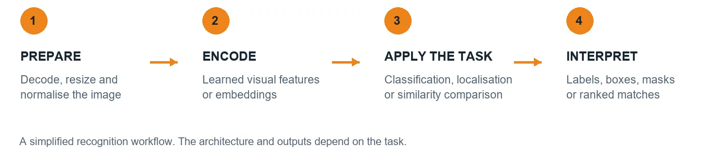
Before prediction, software decodes the image and prepares the input expected by the model. Preparation may include resizing, cropping, converting the colour format, and scaling or normalising values. The exact recipe depends on how that model was trained. An image that looks correct on your screen can still be an unsuitable numerical input if its preparation is wrong.
Resizing also makes a practical trade-off. Smaller inputs need less computation, but a tiny distant bicycle may lose the details that distinguish it from a railing. Preparation is already part of what the system can perceive.
Learning happens before your search
In supervised training, examples come with targets. A classification dataset might pair photographs with labels such as “bicycle” or “boat.” The model predicts an answer, a loss function measures its error, and an optimisation procedure adjusts its internal parameters. Repeating this across examples gradually changes which patterns influence its predictions. 1
The labels define the training task; they are not little explanations of each picture. A bicycle label does not explicitly teach wheels, balance, transportation, or why somebody parked beside the sea. The model must find useful statistical patterns in the examples it receives.
Evaluation uses held-out examples to check whether that learning transfers beyond the training pictures. If the same or nearly identical photographs appear on both sides, the result can give an exaggerated impression of performance.
Inference is the later stage when a trained model processes a new image. In ordinary inference, its learned parameters stay fixed. Searching your holiday album does not, by itself, mean the underlying model is being retrained on that album. 1
Labelled classification is one training approach. Other systems learn from image–text pairs, as we will see with CLIP.
Two ways to find visual patterns
There is no single mechanism behind every image model. Convolutional neural networks and Vision Transformers provide two useful examples.
Convolutional networks examine local patterns
A convolutional neural network, or CNN, applies learned filters across small regions. Each filter combines nearby values using the same set of weights at different locations, producing a feature map. Early filters can respond to patterns such as edges or colour contrasts; later layers combine information from wider regions. 2
Imagine the repeated curves and spokes in a bicycle photo. A network can use combinations of visual responses to support a bicycle prediction. This is an illustration, however, not a promise that every layer corresponds neatly to “edge,” then “wheel,” then “bicycle.” Internal features are often harder to name.
Vision Transformers connect image patches
The original Vision Transformer, or ViT, divides an image into patches and converts each patch into a vector of numbers. Position information helps retain where patches came from. Self-attention then allows their representations to exchange information across the image. 3
For a 224 × 224 image divided into non-overlapping 16 × 16 patches, there are 224 ÷ 16 = 14 patches along each side, giving 14 × 14 = 196 patch tokens. Each RGB patch starts with 16 × 16 × 3 = 768 values before its learned projection.
In the original classification design, an additional classification token brings the sequence to 197 tokens. Other designs can use different resolutions, patch sizes, or extra tokens, so 196 is an example, not a universal image-token count. 3
Both approaches can produce learned visual features. What happens next depends on the question the system was designed to answer.
Different questions need different outputs
Recognising that a bicycle appears somewhere in a photograph is different from locating its handlebars or separating it from the background. A task head is the part of a model that turns learned features into the required output. Detection and segmentation systems retain spatial information so they can make predictions about locations. 4
| Task | Question | Example output |
|---|---|---|
| Classification | What category fits this image? | “Bicycle” or several image labels |
| Object detection | What objects are present, and where? | Boxes around two bicycles |
| Semantic segmentation | What category belongs to each pixel? | Bicycle pixels separated from road pixels |
| Instance segmentation | Which pixels belong to each individual object? | A separate mask for each bicycle |
A box is a convenient boundary, while a mask follows an object's visible outline more closely. Semantic segmentation groups by category; instance segmentation distinguishes separate objects within that category. These distinctions matter when choosing a tool: an album tagger and a background-removal tool need different outputs. 4
Embeddings make similarity searchable
An embedding represents an image as a vector whose relationships to other vectors are useful for a learned task. Think of it as coordinates in a space with many dimensions, rather than a written description hidden inside the picture.
CLIP learns image and text representations together. Its training encourages matching image–text pairs to have higher similarity than mismatched pairs. At search time, a system can compare the embedding of “a bicycle beside the sea” with embeddings of candidate photographs, often using cosine similarity, which compares vector directions. 5
This makes language-based retrieval possible without requiring someone to manually assign that exact phrase to every photograph. It also introduces a limit: a strong match is a learned association, not proof of complete human-like understanding. Wording and the choice of candidate descriptions can affect the result. 5
Our imaginary album search therefore returns promising candidates. You still decide whether a particular photo actually shows the scene you had in mind.
Describing a picture and making one are different tasks
Image captioning combines visual information with language generation. An image-conditioned language model produces a sequence of words intended to describe the input. The early Show and Tell research demonstrated this connection between a visual representation and a sentence-generating model. 6
Multimodal systems can also accept a picture together with a question. “What is beside the bicycle?” requires a language response grounded in the image. This differs from CLIP-style retrieval, which compares representations and ranks candidates rather than independently composing a caption.
Image generation produces an image as its output. A diffusion model, for example, learns a denoising process and can generate a sample by progressively transforming noise. Text-conditioned versions use a prompt to guide generation. 7
The concepts can overlap within larger systems, but a tool that labels a photograph does not automatically know how to create one. Equally, an attractive generated picture is not evidence that a system correctly interpreted a supplied photograph.
Why a convincing answer can still be wrong
Training data shapes what becomes familiar. If a hypothetical dataset mostly shows bicycles outdoors, the model may over-rely on outdoor backgrounds. This is one possible form of dataset bias. Uneven coverage can also leave everyday objects, environments, or cultural contexts poorly represented. A large dataset alone does not establish that every group or situation receives equally reliable performance.
Domain shift occurs when the images encountered in use differ from those represented during training. A well-lit product photograph and a blurred evening snapshot can depict the same object while presenting quite different signals. Research on common image corruptions shows why noise, blur, and weather-like changes deserve explicit testing. 8
A confidence score also needs interpretation. Calibration asks whether stated probabilities match observed correctness over many relevant examples. Among predictions given about 80% confidence, a calibrated system should be right about 80% of the time. That is a population-level property, not a guarantee for one image, and neural-network scores can be poorly calibrated. 9
Captioning introduces another failure: hallucination. A model may mention something absent from the image because it commonly appears in similar descriptions. Research has found that better scores on standard caption metrics do not necessarily mean fewer invented objects. A fluent sentence needs checking against the actual picture. 10
Human validation should match the consequence of an error. A mistaken holiday tag is easy to fix. An inspection decision affecting a product shipment deserves a defined review process, relevant evaluation examples, and a way to flag uncertain results.
Try changing one thing at a time
You can explore these ideas with a mug, a spoon, and a toy car. Photograph them against a plain background, keeping people, private documents, and identifying details out of frame. Use an image-classification or captioning tool you already have access to, and record its answer for each original image.
Next, change one condition: dim the light, turn the object, move it onto a patterned cloth, or partially cover it. Keep the task and wording fixed. Compare the original and altered results, including confidence scores if the tool exposes them.
If a mug becomes a bowl when its handle disappears, you have a useful observation to investigate. If a caption invents a tablecloth pattern, you have a grounding error to record. Neither observation alone reveals exactly how the model reasoned, and a few examples cannot establish general accuracy.
The experiment makes the central idea tangible. AI vision turns visual measurements into learned representations and task-specific predictions. Its usefulness grows when we understand what the output means, test the conditions it will encounter, and leave room to check the answer.
Sources and further reading
Specifications, research papers and official documentation support the technical explanations. The examples and diagrams are original editorial material. Research checked on 23 October 2026.
- PyTorch Quickstart — Official walkthrough of datasets, labels, optimisation, evaluation, and prediction with a trained model.
- Stanford CS231n Convolutional Neural Networks — Course notes explaining image arrays, shared convolutional filters, feature maps, and CNN layers.
- An Image is Worth 16x16 Words — Original Vision Transformer paper supporting patches, position embeddings, attention, and the additional classification token.
- TorchVision Object Detection Finetuning Tutorial — Official example explaining object labels, bounding boxes, instance masks, and task-specific prediction components.
- Learning Transferable Visual Models From Natural Language Supervision — Original CLIP paper describing paired image–text learning, embeddings, cosine similarity, transfer, and limitations.
- Show and Tell A Neural Image Caption Generator — Primary research connecting image representations with generated natural-language descriptions.
- High-Resolution Image Synthesis with Latent Diffusion Models — Primary research on diffusion image synthesis, denoising in latent space, and text-conditioned generation.
- Benchmarking Neural Network Robustness to Common Corruptions and Perturbations — Primary research testing image classifiers under common corruptions and perturbations.
- On Calibration of Modern Neural Networks — Primary research distinguishing confidence scores from empirically reliable probabilities.
- Object Hallucination in Image Captioning — Primary research on absent objects in generated captions and limits of standard caption metrics.